深度学习原理：循环神经网络RNN和LSTM网络结构、结构变体(peephole,GRU)、前向传播公式以及TF实现简单解析

循环神经网络背景这里先不介绍了。本文暂时先记录RNN和LSTM的原理。

首先RNN。RNN和LSTM都是参数复用的，然后每个时间步展开。

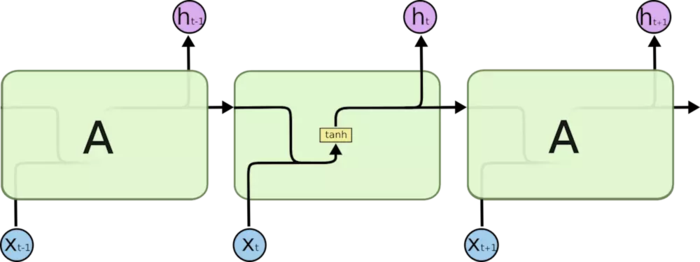
RNN的cell比较简单，我们用Xt表示t时刻cell的输入，Ct表示t时刻cell的状态，ht表示t时刻的输出（输出和状态在RNN里是一样的）。

那么其前向传播的公式也很简单：$h_t=C_t=[h_{t-1},X_t]*W+b$

其中[,]表示concat。W和b分别为RNN的kernel和bias。

然后LSTM，是RNN的升级版，加入了forget、input、output三个门，包含3个门，5对参数，两次更新。赋予了RNN选择性记忆的能力，一定程度解决了RNN中Long Term Dependency（长期依赖）的问题。

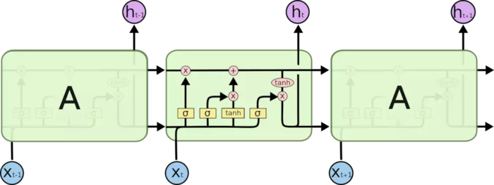
从左向右，三个sigmoid分别对应三个门：forget,input,output，后面用f,i,o代替。

按从左至右顺序：

首先是forget gate：$f_t=sigma([h_{t-1},X_t]*W_f+b_f)$

forget gate用sigmoid函数激活，得到一个0~1的数，来决定$S_{t-1}$的“记忆”留着哪些，忘记哪些。剩下两个gate用法也类似。

然后是input gate:$i_t=sigma([h_{t-1},X_t]*W_i+b_i)$

更新细胞状态C:$C_t=f_totimes C_{t-1}+i_totimes tanh(([h_{t-1},X_t]*W_s+b_s)$

之后是output gate:$o_t=sigma([h_{t-1},X_t]*W_o+b_o)$

最后更新输出h:$h_t=o_totimes tanh(C_{t})$

整个流程大概就这样，方便记忆，我们可以把前向公式整理成下面顺序：

$f_t=sigma([h_{t-1},X_t]*W_f+b_f)$

$i_t=sigma([h_{t-1},X_t]*W_i+b_i)$

$o_t=sigma([h_{t-1},X_t]*W_o+b_o)$

$C_t=f_totimes C_{t-1}+i_totimes tanh(([h_{t-1},X_t]*W_s+b_s)$

$h_t=o_totimes tanh(C_{t})$

可以方便的看出5对参数（kernel+bias），3个门，2次更新。

以上是LSTM比较通用的原理，在tensorflow实现中，和上面略有不同，稍微做了简化。

具体源码可参见：https://github.com/tensorflow/tensorflow/blob/r1.12/tensorflow/python/ops/rnn_cell_impl.py  L165：BasicLSTMCell

源码延续了f,i,o,c,h的表示

    #build
    self._kernel = self.add_variable(
        _WEIGHTS_VARIABLE_NAME,
        shape=[input_depth + h_depth, 4 * self._num_units])
    self._bias = self.add_variable(
        _BIAS_VARIABLE_NAME,
        shape=[4 * self._num_units],
        initializer=init_ops.zeros_initializer(dtype=self.dtype))

    gate_inputs = math_ops.matmul(
        array_ops.concat([inputs, h], 1), self._kernel)
    gate_inputs = nn_ops.bias_add(gate_inputs, self._bias)

    # i = input_gate, j = new_input, f = forget_gate, o = output_gate
    i, j, f, o = array_ops.split(
        value=gate_inputs, num_or_size_splits=4, axis=one)

在build方法中，将门和状态更新的参数们一起定义了。后面在call方法中，直接相乘再给split开，化简了操作。

    forget_bias_tensor = constant_op.constant(self._forget_bias, dtype=f.dtype)
    # Note that using `add` and `multiply` instead of `+` and `*` gives a
    # performance improvement. So using those at the cost of readability.
    add = math_ops.add
    multiply = math_ops.multiply
    new_c = add(multiply(c, sigmoid(add(f, forget_bias_tensor))),
                multiply(sigmoid(i), self._activation(j)))
    new_h = multiply(self._activation(new_c), sigmoid(o))

之后在更新操作中，将该用sigmoid的三个门的激活函数写死，两个更新操作的激活函数则随LSTM初始化参数改变。并多加了一个forget_bias_tensor，这个和原LSTM原理略有不同。

 

除此之外，LSTM还有几种变体：

1.peephole connection:

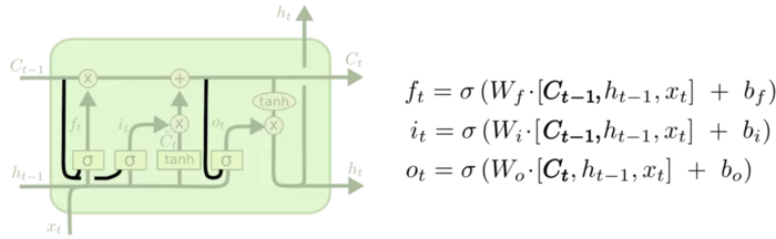
思路很简单，也就是我们让 门层 也会接受细胞状态的输入。

其他没有改变。注意outputgate接受的是更新后的细胞状态。

2.coupled

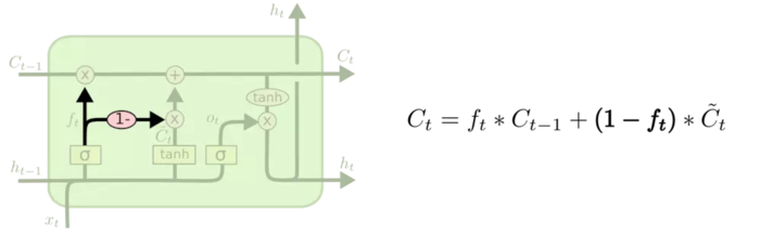
思路也很简单

inputgate forgetgate复用一个门，其他一样。

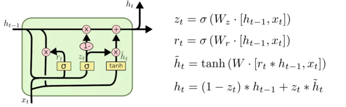
3.GRU

Gated Recurrent Unit (门控循环单元，GRU)是一个改动比较大的变体。这是由 Cho, et al. (2014) 提出。它将忘记门和输入门合成了一个单一的 更新门。同样还混合了细胞状态和隐藏状态，和其他一些改动。最终的模型比标准的 LSTM 模型要简单，也是非常流行的变体。

 

 

 

 

参考资料：

https://www.jianshu.com/p/9dc9f41f0b29