An overview of object detection: one-stage methods 目标检测概述:一步法
(点击标题链接原文https://www.jeremyjordan.me/object-detection-one-stage/)
Object detection is useful for understanding what’s in an image, describing both what is in an image and where those objects are found.
目标检测是了解什么是图像中,描述都是有用的东西是一个图像并在那里被发现的那些对象。
In general, there’s two different approaches for this task – we can either make a fixed number of predictions on grid (one stage) or leverage a proposal network to find objects and then use a second network to fine-tune these proposals and output a final prediction (two stage).
一般来说,这项任务有两种不同的方法:
- 我们既可以在网格上进行固定数量的预测(一个阶段),
- 也可以利用提案网络查找对象,然后使用第二个网络对这些提案进行微调并输出最终结果预测(两阶段)。
Each approach has its own strengths and weaknesses
每种方法都有自己的优点和缺点
Understanding the task 理解任务
The goal of object detection is to recognize instances of a predefined set of object classes (e.g. {people, cars, bikes, animals}) and describe the locations of each detected object in the image using a bounding box.
目标检测的目标是识别预定义的一组对象类(例如{人,汽车,自行车,动物})的实例,并使用边界框描述图像中每个检测到的对象的位置。

We’ll use rectangles to describe the locations of each object. An alternative approach would be image segmentation which provides localization at the pixel-level.
我们将使用矩形来描述每个对象的位置。另一种方法是图像分割,其提供像素级的定位。
Direct object prediction 直接对象预测
This blog post will focus on model architectures which directly predict object bounding boxes for an image in a one-stage fashion.
这篇博文将重点介绍模型体系结构,它以一阶段的方式直接预测图像的对象边界框。
Predictions on a grid 对网络的预测
We’ll refer to this part of the architecture as the “backbone” network, which is usually pre-trained as an image classifier to more cheaply learn how to extract features from an image.
我们将架构的这一部分称为“骨干”网络,它通常被预先训练为图像分类器,以便更便宜地学习如何从图像中提取特征。
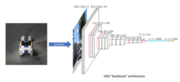
After pre-training the backbone architecture as an image classifier, we’ll remove the last few layers of the network so that our backbone network outputs a collection of stacked feature maps which describe the original image in a low spatial resolution albeit a high feature (channel) resolution.
在将骨干架构作为图像分类器进行预训练之后,我们将删除网络的最后几层,以便我们的骨干网络输出一组堆叠的特征图,这些图以低空间分辨率描述原始图像,尽管具有高特征(频道)决议。
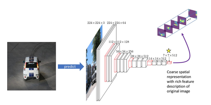
Coarse spatial representation with rich feature description of original image
原始图像特征丰富描述和粗糙空间表示
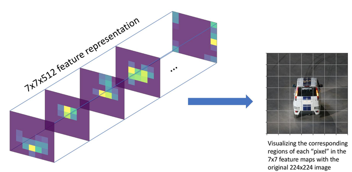
We can relate this 7x7 grid back to the original input in order to understand what each grid cell represents relative to the original image.
我们可以将这个7x7网格与原始输入相关联,以便了解每个网格单元相对于原始图像的表示。
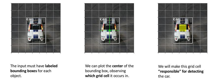
We can also determine roughly where objects are located in the coarse (7x7) feature maps by observing which grid cell contains the center of our bounding box annotation. We’ll assign this grid cell as being “responsible” for detecting that specific object.
我们还可以通过观察哪个网格单元包含我们的边界框注释的中心来粗略地确定对象在粗(7x7)要素图中的位置。我们将此网格单元指定为“负责”以检测该特定对象。
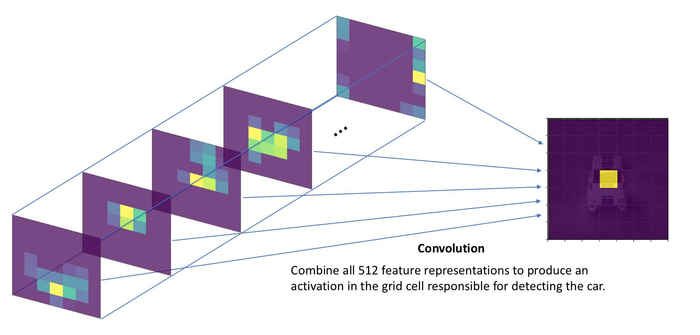
In order to detect this object, we will add another convolutional layer and learn the kernel parameters which combine the context of all 512 feature maps in order to produce an activation corresponding with the grid cell which contains our object.
为了检测这个对象,我们将添加另一个卷积层并学习内核参数,这些参数组合了所有512个特征映射的上下文,以便产生与包含我们对象的网格单元相对应的**。
If the input image contains multiple objects, we should have multiple activations on our grid denoting that an object is in each of the activated regions.
如果输入图像包含多个对象,我们应该在网格上进行多次**,表示对象位于每个**区域中。
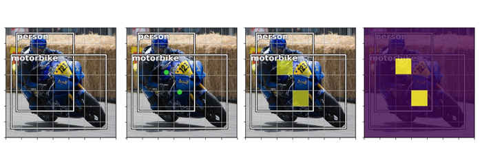
However, we cannot sufficiently describe each object with a single activation. In order to fully describe a detected object, we’ll need to define:
但是,我们无法通过单次**来充分描述每个对象。为了完整描述检测到的对象,我们需要定义:
- The likelihood that a grid cell contains an object \( (p_{obj}) \)
- 网络单元包含对象的可能性\( (p_{obj}) \)
- Which class the object belongs to \( (c_1, c_2, …, c_C) \)
- 对象属于哪个类\( (c_1, c_2, …, c_C) \)
- Four bounding box descriptors to describe the x coordinate, y coordinate, width, and height of a labeled box \( (t_x, t_y, t_w, t_h) \)
- 用于描述四个边界框,坐标x,坐标y,标记框的宽度和高度\( (t_x, t_y, t_w, t_h) \)
Thus, we’ll need to learn a convolution filter for each of the above attributes such that we produce 5+C output channels to describe a single bounding box at each grid cell location. This means that we’ll learn a set of weights to look across all 512 feature maps and determine which grid cells are likely to contain an object, what classes are likely to be present in each grid cell, and how to describe the bounding box for possible objects in each grid cell.
因此,我们需要为每个上述属性学习卷积滤波器,以便生成5 + C.输出通道来描述每个网格单元位置的单个边界框。这意味着我们将学习一组权重来查看所有512个要素图并确定哪些网格单元可能包含对象,每个网格单元中可能存在哪些类,以及如何描述边界框每个网格单元中的可能对象。
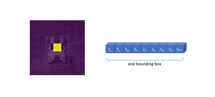
The full output of applying 5+C convolutional filters is shown below for clarity, producing one bounding box descriptor for each grid cell.
应用5 + C的完整输出 为清楚起见,下面显示了卷积滤波器,为每个网格单元生成一个边界框描述符。

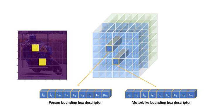
However, some images might have multiple objects which “belong” to the same grid cell. We can alter our layer to produce B(5+C) filters such that we can predict B bounding boxes for each grid cell location.
但是,某些图像可能具有多个“属于”同一网格单元的对象。我们可以改变我们的层来生产B (5 + C.)我们可以预测B过滤器 每个网格单元位置的边界框。

Visualizing the full convolutional output of our B(5+C) filters, we can see that our model will always produce a fixed number of N×N×B predictions for a given image. We can then filter our predictions to only consider bounding boxes which has a \( p_{obj} \) above some defined threshold.
可视化我们B的完整卷积输出(5 + C.)过滤器,我们可以看到我们的模型将始终产生固定数量的N.× N× B对给定图像的预测。然后我们可以过滤我们的预测,只考虑具有p的边界框 \( p_{obj} \) 高于某个定义的阈值。

Because of the convolutional nature of our detection process, multiple objects can be detected in parallel. However, we also end up predicting for a large number grid cells where no object is found. Although we can filter these bounding boxes out by their \( p_{obj} \) score, this introduces quite a large imbalance between the predicted bounding boxes which contain an object and those which do not contain an object.
由于检测过程的卷积性质,可以并行检测多个对象。但是,我们最终还会预测没有找到对象的大量网格单元。虽然我们可以通过p来过滤这些边界框 \( p_{obj} \) 得分,这在包含对象的预测边界框和不包含对象的边界框之间引入了相当大的不平衡。
The two models I’ll discuss below both use this concept of “predictions on a grid” to detect a fixed number of possible objects within an image. In the respective sections, I’ll describe the nuances of each approach and fill in some of the details that I’ve glanced over in this section so that you can actually implement each model.
我将在下面讨论的两个模型都使用“网格预测”的概念来检测图像中固定数量的可能对象。在相应的部分中,我将描述每种方法的细微差别,并填写我在本节中瞥过的一些细节,以便您可以实际实现每个模型。
非最大抑制
The “predictions on a grid” approach produces a fixed number of bounding box predictions for each image.
“对网格的预测”方法为每个图像产生固定数量的边界框预测。
we need a method for removing redundant object predictions such that each object is described by a single bounding box.
我们需要一种用于移除冗余对象预测的方法,使得每个对象由单个边界框描述。
To accomplish this, we’ll use a technique known as non-max suppression. At a high level, this technique will look at highly overlapping bounding boxes and suppress (or discard) all of the predictions except the highest confidence prediction.
为此,我们将使用一种称为非最大抑制的技术。在高层次上,该技术将查看高度重叠的边界框并抑制(或丢弃)除最高置信度预测之外的所有预测。
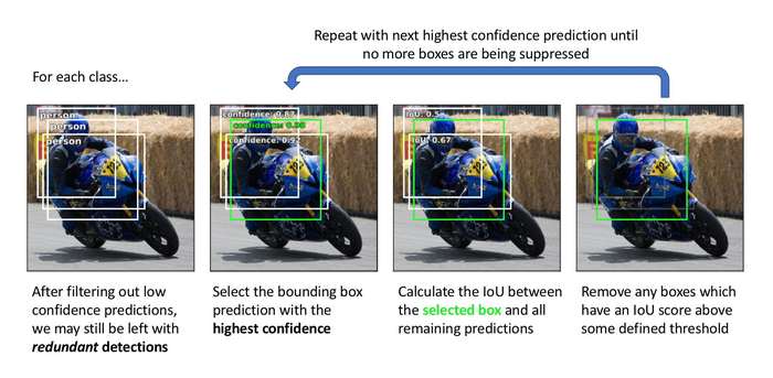
We’ll perform non-max suppression on each class separately. Again, the goal here is to remove redundant predictions so we shouldn’t be concerned if we have two predictions that overlap if one box is describing a person and the other box is describing a bicycle. However, if two bounding boxes with high overlap are both describing a person, it’s likely that these predictions are describing the same person.
我们将分别对每个类执行非最大抑制。同样,这里的目标是删除多余的预测,因此如果我们有两个预测重叠,如果一个框描述一个人而另一个框描述自行车,我们就不应该担心。但是,如果两个具有高重叠的边界框都描述了一个人,那么这些预测很可能描述的是同一个人。
YOLO: You Only Look Once YOLO:你只看一次
The YOLO model was first published (by Joseph Redmon et al.) in 2015 and subsequently revised in two following papers. In each section, I’ll discuss the specific implementation details and refinements that were made to improve performance.
YOLO模型于2015年首次发布(作者Joseph Redmon等人),随后在以下两篇论文中进行了修订。在每个部分中,我将讨论为提高性能而制定的具体实现细节和改进。
Backbone network 骨干网
The original YOLO network uses a modified GoogLeNet as the backbone network. His latest paper introduces a new, larger model named DarkNet-53 which offers improved performance over its predecessor.
最初的YOLO网络使用经过修改的GoogLeNet作为骨干网络。他的最新论文介绍了一款名为DarkNet-53的新型大型机型,该机型比其前代机型具有更高的性能。
In the second iteration of the YOLO model, Redmond discovered that using higher resolution images at the end of classification pre-training improved the detection performance and thus adopted this practice.
在YOLO模型的第二次迭代中,Redmond发现在分类预训练结束时使用更高分辨率的图像可以提高检测性能,从而采用这种方法。
Bounding boxes (and concept of anchor boxes) 边界框(和锚箱的概念)
The first iteration of the YOLO model directly predicts all four values which describe a bounding box. The x and y coordinates of each bounding box are defined relative to the top left corner of each grid cell and normalized by the cell dimensions such that the coordinate values are bounded between 0 and 1. We define the boxes width and height such that our model predicts the square-root width and height; by defining the width and height of the boxes as a square-root value, differences between large numbers are less significant than differences between small numbers (confirm this visually by looking at a plot of \( y = \sqrt{x} \) ). calculating our loss function we would like the emphasis to be placed on getting small boxes more exact.
YOLO模型的第一次迭代直接预测描述边界框的所有四个值。该X和y每个边界框的坐标相对于每个网格单元的左上角定义,并由单元尺寸标准化,使得坐标值在0和1之间限定。我们定义框的宽度和高度,以便我们的模型预测方形 -根宽和高度; 通过将方框的宽度和高度定义为平方根值,大数字之间的差异不如小数字之间的差异显着(通过查看y的图表在视觉上确认\( y = \sqrt{x} \) )。重点放在更精确地获得小盒子上。
Redmond offers an approach towards discovering the best aspect ratios by doing k-means clustering (with a custom distance metric) on all of the bounding boxes in your training dataset.
Redmond提供了一种方法,通过在训练数据集中的所有边界框上执行k均值聚类(使用自定义距离度量)来发现最佳宽高比。
In the image below, you can see a collection of 5 bounding box priors (also known as anchor boxes) for the grid cell highlighted in yellow. With this formulation, each of the B bounding boxes explicitly specialize in detecting objects of a specific size and aspect ratio.
在下图中,您可以看到以黄色突出显示的网格单元的5个边界框先验(也称为锚框)的集合。用这个配方,每个B 边界框明确专门用于检测特定大小和宽高比的对象。
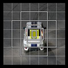
Note: Although it is not visualized, these anchor boxes are present for each cell in our prediction grid.
注意:虽然它不可视化,但我们的预测网格中的每个单元格都存在这些锚框。
Rather than directly predicting the bounding box dimensions, we’ll reformulate our task in order to simply predict the offset from our bounding box prior dimensions such that we can fine-tune our predicted bounding box dimensions. This reformulation makes the prediction task easier to learn.
我们不是直接预测边界框尺寸,而是重新构造我们的任务,以便简单地预测我们的边界框先前维度的偏移量,以便我们可以微调我们预测的边界框尺寸。这种重新制定使预测任务更容易学习。
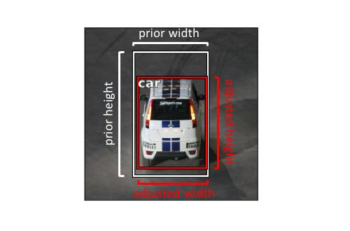
For similar reasons as originally predicting the square-root width and height, we’ll define our task to predict the log offsets from our bounding box prior.
由于与最初预测平方根宽度和高度相似的原因,我们将定义我们的任务,以预先确定来自边界框的日志偏移。
Objectness (and assigning labeled objects to a bounding box) 对象(并将标记的对象分配给边界框)
YOLOv1
the “objectness” score \( p_{obj} \) was trained to approximate the Intersection over Union (IoU) between the predicted box and the ground truth label. When we calculate our loss during training, we’ll match objects to whichever bounding box prediction (on the same grid cell) has the highest IoU score.
“对象性”得分为\( p_{obj} \)被训练以近似预测的框和地面真实标签之间的联合交叉(IoU)。当我们在训练期间计算我们的损失时,我们将对象与任何边界框预测(在同一网格单元格上)具有最高IoU分数的对象匹配。
YOLOv2
we can simply assign labeled objects to whichever anchor box (on the same grid cell) has the highest IoU score with the labeled object.
添加边界框之前,我们可以简单地将标记对象分配给具有标记对象的最高IoU分数的任何锚框(在同一网格单元格上)。
YOLOv3
In the third version, Redmond redefined the “objectness” target score \( p_{obj} \) to be 1 for the bounding boxes with highest IoU score for each given target, and 0 for all remaining boxes. However, we will not include bounding boxes which have a high IoU score (above some threshold) but not the highest score when calculating the loss. In simple terms, it doesn’t make sense to punish a good prediction just because it isn’t the best prediction.
雷德蒙德重新定义了“对象性”目标得分\( p_{obj} \)对于每个给定目标具有最高IoU分数的边界框为1,对于所有剩余框具有0。但是,在计算损失时,我们不会包含具有高IoU分数(高于某个阈值)但不是最高分数的边界框。简单来说,仅仅因为它不是最好的预测而惩罚好的预测是没有意义的。
Class labels 类标签
predict class for each bounding box using a softmax activation across classes and a cross entropy loss.
使用跨类的softmax**和交叉熵损失来预测每个边界框的类。
use sigmoid activations for multi-label classification
使用sigmoid**进行多标签分类
Output layer 输出层
The first YOLO model simply predicts the N×N×B bounding boxes using the output of our backbone network.
第一个YOLO模型简单地预测N.× N× B 使用我们的骨干网络输出的边界框。
In YOLOv2, Redmond adds a weird skip connection splitting a higher resolution feature map across multiple channels as visualized below.
在YOLOv2中,Redmond添加了一个奇怪的跳过连接,将更高分辨率的特征映射分成多个通道,如下图所示。

This was changed in the third iteration for a more standard feature pyramid network output structure. With this method, we’ll alternate between outputting a prediction and upsampling the feature maps (with skip connections). This allows for predictions that can take advantage of finer-grained information from earlier in the network, which helps for detecting small objects in the image.
这在第三次迭代中被更改为更标准的功能金字塔网络输出结构。使用此方法,我们将在输出预测和上采样特征映射(使用跳过连接)之间进行交替。这允许预测可以利用来自网络早期的更细粒度的信息,这有助于检测图像中的小对象。

SSD: Single Shot Detection SSD:单次检测
The SSD model was also published (by Wei Liu et al.) in 2015
SSD模型也于2015年发布(由Wei Liu等人发布)
Backbone network 骨干网
A VGG-16 model, pre-trained on ImageNet for image classification, is used as the backbone network. The authors make a few slight tweaks when adapting the model for the detection task, including: replacing fully connected layers with convolutional implementations, removing dropout layers, and replacing the last max pooling layer with a dilated convolution.
在ImageNet上预先训练用于图像分类的VGG-16模型用作骨干网络。作者在为检测任务调整模型时进行了一些微调,包括:用卷积实现替换完全连接的层,删除丢失层,并用扩散卷积替换最后一个最大池层。
Bounding boxes (and concept of anchor boxes) 边界框(和锚箱的概念)
SSD model manually defines a collection of aspect ratios (eg. {1, 2, 3, 1/2, 1/3}) to use for the B bounding boxes at each grid cell location.
SSD模型手动定义的纵横比的集合(例如,{1,2,3,1/2,1/3})要使用的乙 每个网格单元位置的边界框。
For each bounding box, we’ll predict the offsets from the anchor box for both the bounding box coordinates (x and y) and dimensions (width and height). We’ll use ReLU activations trained with a Smooth L1 loss.
对于每个边界框,我们将预测边界框坐标(x。)的锚点偏移量和y)和尺寸(宽度和高度)。我们将使用受到平滑L1损失训练的ReLU**。
Objectness (and assigning labeled objects to a bounding box) 对象(并将标记的对象分配给边界框)
SSD does not attempt to predict a value for \( p_{obj} \).SSD model attempts to directly predict the probability that a class is present in a given bounding box.
SSD 不会尝试预测\( p_{obj} \)。SSD模型试图直接预测在给定的边界框中存在类的概率。
When calculating the loss, we’ll match each ground truth box to the anchor box with the highest IoU — defining this box with being “responsible” for making the prediction.
在计算损失时,我们将每个地面实况框与具有最高IoU的锚框匹配 - 定义此框以“负责”进行预测。
Class labels 类标签
we directly predict the probability of each class using a softmax activation and cross entropy loss.
使用softmax**和交叉熵损失直接预测每个类的概率。
Due to the fact that most of the boxes will belong to the “background” class, we will use a technique known as “hard negative mining” to sample negative (no object) predictions such that there is at most a 3:1 ratio between negative and positive predictions when calculating our loss.
由于大多数盒子都属于“背景”类,我们将使用一种称为“硬阴性采矿”的技术来对负(无对象)预测进行采样,使得之间的比率最多为3:1。计算损失时的负面和正面预测。
Output layer 输出层
The SSD output module progressively downsamples the convolutional feature maps, intermittently producing bounding box predictions (as shown with the arrows from convolutional layers to the predictions box).
SSD输出模块逐步对卷积特征图进行下采样,间歇地产生边界框预测(如从卷积层到预测框的箭头所示)。

Addressing object imbalance with focal loss 通过焦点丢失解决物体不平衡问题
Researchers at Facebook proposed adding a scaling factor to the standard cross entropy loss such that it places more the emphasis on “hard” examples during training, preventing easy negative predictions from dominating the training process.
Facebook的研究人员建议在标准交叉熵损失中增加一个比例因子,以便在训练期间更多地强调“硬”例子,防止容易的负面预测主导训练过程。
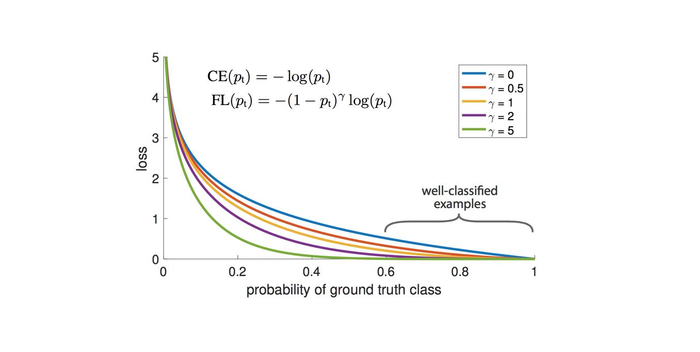
As the researchers point out, easily classified examples can incur a non-trivial loss for standard cross entropy loss \( (\gamma = 0) \) which, summed over a large collection of samples, can easily dominate the parameter update. The \( (1−p_t)^\gamma \) term acts as a tunable scaling factor to prevent this from occuring.
正如研究人员指出的那样,容易分类的例子可能会导致标准交叉熵损失的重大损失\( (\gamma = 0) \),对大量样本进行求和,可以很容易地控制参数更新。所述\( (1−p_t)^\gamma \)作为可调整的缩放因子来防止这种情况发生。
As the paper points out, “with \( (\gamma = 2) \), an example classified with \( p_t= 0.9 \) would have 100X lower loss compared with CE and with \( p_t=0.968 \) it would have 1000X lower loss.”
正如文章所指出的那样,“用\( (\gamma = 2) \),一个用p分类的例子\( p_t= 0.9 \)与CE和p相比,损失将减少100倍\( p_t= 0.968 \) 它的损失会低1000倍。“
Common datasets and competitions 常见数据集和竞赛
下面我列出了研究人员在评估新物体检测模型时使用的一些常见数据集。
Further reading 进一步阅读
论文
-
YOLO
-
SSD
-
DSSD: Deconvolutional Single Shot Detector (I didn’t discuss this in the blog post but it’s worth the read)
-
讲座
-
博客文章
-
框架和GitHub
-
用于标记数据的工具
本站文章如无特殊说明,均为本站原创,如若转载,请注明出处:目标检测概述:一步法 An overview of object detection: one-stage methods - Python技术站

 微信扫一扫
微信扫一扫  支付宝扫一扫