Time series prediction (forecasting) has experienced dramatic improvements in predictive accuracy as a result of the data science machine learning and deep learning evolution. As these ML/DL tools have evolved, businesses and financial institutions are now able to forecast better by applying these new technologies to solve old problems. In this article, we showcase the use of a special type of Deep Learning model called an LSTM (Long Short-Term Memory), which is useful for problems involving sequences with autocorrelation. We analyze a famous historical data set called “sunspots” (a sunspot is a solar phenomenon wherein a dark spot forms on the surface of the sun). We’ll show you how you can use an LSTM model to predict sunspots ten years into the future with an LSTM model.
TUTORIAL OVERVIEW
This code tutorial goes along with a presentation on Time Series Deep Learning given to SP Globalon Thursday, April 19, 2018. The slide deck that complements this article is available for download.
This is an advanced tutorial implementing deep learning for time series and several other complex machine learning topics such as backtesting cross validation. For those seeking an introduction to Keras in R, please check out Customer Analytics: Using Deep Learning With Keras To Predict Customer Churn.
In this tutorial, you will learn how to:
- Develop a Stateful LSTM Model with the
keraspackage, which connects to the R TensorFlow backend. - Apply a Keras Stateful LSTM Model to a famous time series, Sunspots.
- Perform Time Series Cross Validation using Backtesting with the
rsamplepackage rolling forecast origin resampling. -
Visualize Backtest Sampling Plans and Prediction Results with
ggplot2andcowplot. - Evaluate whether or not a time series may be a good candidate for an LSTM model by reviewing the Autocorrelation Function (ACF) plot.
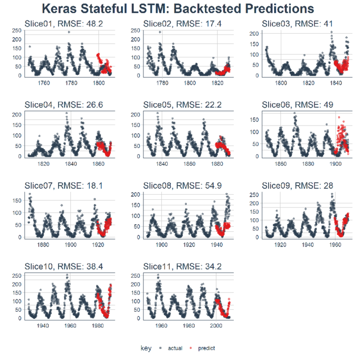
The end result is a high performance deep learning algorithm that does an excellent job at predicting ten years of sunspots! Here’s the plot of the Backtested Keras Stateful LSTM Model.

APPLICATIONS IN BUSINESS
Time series prediction (forecasting) has a dramatic effect on the top and bottom line. In business, we could be interested in predicting which day of the month, quarter, or year that large expenditures are going to occur or we could be interested in understanding how the consumer price index (CPI) will change over the course of the next six months. These are common questions that impact organizations both on a microeconomic and macroeconomic level. While the data set used in this tutorial is not a “business” data set, it shows the power of the tool-problem fit, meaning that using the right tool for the job can offer tremendous improvements in accuracy. The net result is increased prediction accuracy ultimately leads to quantifiable improvements to the top and bottom line.
LONG SHORT-TERM MEMORY (LSTM) MODELS
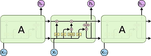
A Long Short-Term Memory (LSTM) model is a powerful type of recurrent neural network (RNN). The blog article, “Understanding LSTM Networks”, does an excellent job at explaining the underlying complexity in an easy to understand way. Here’s an image depicting the LSTM internal cell architecture that enables it to persist for long term states (in addition to short term), which traditional RNN’s have difficulty with:

Source: Understanding LSTM Networks
LSTMs are quite useful in time series prediction tasks involving autocorrelation, the presence of correlation between the time series and lagged versions of itself, because of their ability to maintain state and recognize patterns over the length of the time series. The recurrent architecture enables the states to persist, or communicate between updates of the weights as each epoch progresses. Further, the LSTM cell architecture enhances the RNN by enabling long term persistence in addition to short term, which is fascinating!
In Keras, LSTM’s can be operated in a “stateful” mode, which according to the Keras documentation:
The last state for each sample at index i in a batch will be used as initial state for the sample of index i in the following batch
In normal (or “stateless”) mode, Keras shuffles the samples, and the dependencies between the time series and the lagged version of itself are lost. However, when run in “stateful” mode, we can often get high accuracy results by leveraging the autocorrelations present in the time series.
We’ll explain more as we go through this tutorial. For now, just understand that LSTM’s can be really useful for time series problems involving autocorrelation and Keras has the capability to create stateful LSTMs that are perfect for time series modeling.
SUNSPOTS DATA SET
Sunspots is a famous data set that ships with R (refer to the datasets library). The dataset tracks sunspots, which are the occurrence of a dark spot on the sun. Here’s an image from NASA showing the solar phenomenon. Pretty cool!

Source: NASA
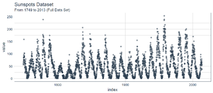
The dataset we use in this tutorial is called sunspots.month, and it contains 265 years (from 1749 through 2013) of monthly data on number of sunspots per month.

IMPLEMENTING AN LSTM TO PREDICT SUNSPOTS
Time to get to business. Let’s predict sunspots. Here’s our objective:
Objective: Use an LSTM model to generate a forecast of sunspots that spans 10-years into the future.
1.0 LIBRARIES
Here are the libraries needed for this tutorial. All are available on CRAN. You can install withinstall.packages() if you do not have them installed already. NOTE: Before proceeding with this code tutorial, make sure to update all packages as previous versions of these packages may not be compatible with the code used. One issue we are aware of is upgrading to lubridateversion 1.7.4.
# Core Tidyverse
library(tidyverse)
library(glue)
library(forcats)

# Time Series
library(timetk)
library(tidyquant)
library(tibbletime)

# Visualization
library(cowplot)

# Preprocessing
library(recipes)

# Sampling / Accuracy
library(rsample)
library(yardstick)

# Modeling
library(keras)
If you have not previously run Keras in R, you will need to install Keras using theinstall_keras() function.
# Install Keras if you have not installed before
install_keras()
2.0 DATA
The dataset, sunspot.month, is available for all of us (it ships with base R). It’s a ts class (not tidy), so we’ll convert to a tidy data set using the tk_tbl() function from timetk. We use this instead of as.tibble() from tibble to automatically preserve the time series index as a zoo yearmonindex. Last, we’ll convert the zoo index to date using lubridate::as_date() (loaded withtidyquant) and then change to a tbl_time object to make time series operations easier.
sun_spots <- datasets::sunspot.month %>%
    tk_tbl() %>%
    mutate(index = as_date(index)) %>%
    as_tbl_time(index = index)

sun_spots
## # A time tibble: 3,177 x 2
## # Index: index
## index value
## <date> <dbl>
## 1 1749-01-01 58.0
## 2 1749-02-01 62.6
## 3 1749-03-01 70.0
## 4 1749-04-01 55.7
## 5 1749-05-01 85.0
## 6 1749-06-01 83.5
## 7 1749-07-01 94.8
## 8 1749-08-01 66.3
## 9 1749-09-01 75.9
## 10 1749-10-01 75.5
## # ... with 3,167 more rows3.0 EXPLORATORY DATA ANALYSIS
The time series is long (265 years!). We can visualize the time series both full (265 years) and zoomed in on the first 50 years to get a feel for the series.
3.1 VISUALIZING SUNSPOT DATA WITH COWPLOT
We’ll make to ggplots and combine them using cowplot::plot_grid(). Note that for the zoomed in plot, we make use of tibbletime::time_filter(), which is an easy way to perform time-based filtering.
p1 <- sun_spots %>%
    ggplot(aes(index, value)) +
    geom_point(color = palette_light()[[1]], alpha = 0.5) +
    theme_tq() +
    labs(
        title = "From 1749 to 2013 (Full Data Set)"
    )

p2 <- sun_spots %>%
    filter_time("start" ~ "1800") %>%
    ggplot(aes(index, value)) +
    geom_line(color = palette_light()[[1]], alpha = 0.5) +
    geom_point(color = palette_light()[[1]]) +
    geom_smooth(method = "loess", span = 0.2, se = FALSE) +
    theme_tq() +
    labs(
        title = "1749 to 1800 (Zoomed In To Show Cycle)",
        caption = "datasets::sunspot.month"
    )

p_title <- ggdraw() +
    draw_label("Sunspots", size = 18, fontface = "bold", colour = palette_light()[[1]])

plot_grid(p_title, p1, p2, ncol = 